
HFSS�쾀�OӋ | PCB�쾀�OӋ��HFSS����������� | HFSS-IE������ʹ��Ԕ����쾀�OӋ����
|
HFSSҕ�l�̳����]�� HFSS��Ӗ�̳����b | ���܌W��HFSS | HFSS����������������� | HFSS���_ɢ�������� HFSS�쾀�OӋ | PCB�쾀�OӋ��HFSS����������� | HFSS-IE������ʹ��Ԕ����쾀�OӋ���� |
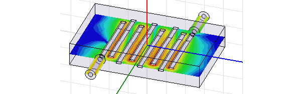
Field overlays are representations of basic or derived field quantities on surfaces or objects for the current design variation. You can set the design variation via the Set Design Variation dialog. This dialog box is accessible from the Solution Data window via by clicking the ellipsis button on the right of the Design Variation field, and via the HFSS or HFSS-IE>Results>Apply Solved Variation command.
You can also overlay existing 3D Polar Plots of near or far fields on the model window by using the HFSS or HFSS-IE>Fields>Plot Fields>Radiation command, or by right-clicking on Field Overlays in the Project tree and selecting Plot Fields>Radiation Field. You can also create animations of field plots.
To plot a basic field quantity:
1. Select a point, line, surface, cutplane, or object to create the plot on or within.
2. Click HFSS or HFSS-IE>Fields>Plot Fields., or right-click on Field Overlay icon in the Project tree and select Plot Fields, or right click in the modeler window, and select Plot Fields from the context menu.
3. On the Plot Fields menu, click the field quantity you want to plot.
The available selections depend on the solved solution. For definitions of the usual quantities, see the list under Quantity command.
If you select a scalar field quantity, a scalar surface or volume plot will be created. If you select a vector field quantity, a vector surface or volume plot will be created. If you select a vector quantity, you will be able to specify a Streamline plot. If the quantity you want to plot is not listed, see Named Expression Library.
For projects with Temperature dependent materials, the HFSS or HFSS-IE>Fields>Plot Fields>Other... menus selections include Temperature.
After you select the field quantity to plot, the Create Field Plot dialog box appears.
The Specify Name field shows a name based on the field quantity you selected, and the Quantity list shows the field quantity selected.
4. To specify a name for the plot other than the default, select Specify Name, and then type a new name in the Name text box.
5. Select the solution to plot from the Solution pull-down list.
6. To specify a folder other than the default in which to store the plot, select Specify Folder, and then click a folder in the Plot Folder pull-down list, or type the name you wish to use. Plot folders are listed under Field Overlays in the project tree. Plot folders let you group plots with the same quantity together. All field plots under the same folder share the same color key.
7. Under Intrinsic Variables, select the frequency and phase angle at which the field quantity is evaluated.
8. If desired, you can select a different field quantity to plot from the Quantity list.
9. Select the volume (region) in which the field will be plotted from the In Volume list.
This selection enables you to limit plots to the intersection of a volume with the selected object or objects. You can select and deselect any items in the In Volume list. You can mix model objects with non-model boxes. For example you might want to see a plot from part of two model objects by restricting the region to a non-model box overlapping those parts.
Note |
Multiple selection should be used when there is a discontinuous field on a surface. If not, the field on both sides of the surface is plotted and each interferes with the other. |
10. If you selected a vector quantity, you can use the checkbox to select Streamline plot. Streamlines are often used to indicate magnetic flux lines, etc. in plots. See Setting Field Plot Attributes for adjusting the streamline display and Setting Fields Reporter Options for setting Streamline defaults.

11. Click Done.
The field quantity is plotted on the surfaces or within the objects you selected. The plot uses the attributes specified in the Plot Attributes dialog box.
The new plot appears in the view window. It is listed in the specified plot folder in the project tree. If you have created a field plot on a simulation in progress, the field plot is updated after the last adaptive solution. Each category of plots (such as Temperature) are listed separately in the Project Tree.

If you want to update the field overlay before then, to view progress in the solution, select the Field icon in the Project tree that contains the field plot of interest, right-click to display the short cut menu, and select Update Plots.
To turn off the display of the plot, right click on the plot and select Plot Visibility from the short-cut menu. Unchecking Plot Visibility turns off the plot display.
Plotting Derived Field Quantities
Overlaying 3D Polar Plots on Models
Selecting the Face or Object Behind
Working with Scalar Field Plot Markers
Technical Notes: Field Overlays
Technical Notes: Field Quantities
Technical Notes: Specifying the Phase Angle

|
||
Ansys HFSS��Ansoft HFSS online help��Version 15.0. |
HFSSҕ�l�̳� | HFSS�̳̌��� | ���l���̎���Ӗ��Ӗ�n�� : Plotting Field Overlays'>HFSSComments |